Background and Template Construction
Background
In the classic formulation of star formation history fitting from resolved-star photometry [1], an observed color-magnitude diagram (CMD) is binned into a 2-D histogram known as a Hess diagram. Such a CMD and Hess diagram pair is shown below.
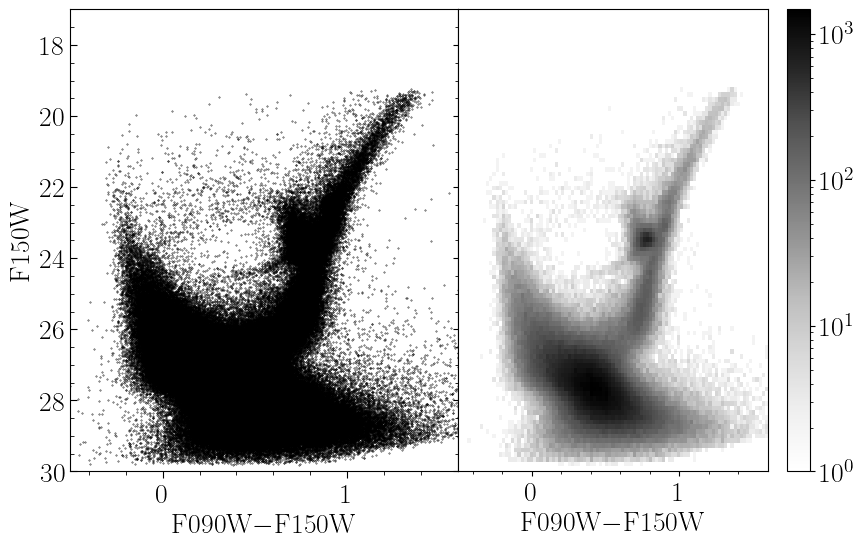
The representation of the observations as a Hess diagram allows one to apply Poisson statistics, specifically the Poisson likelihood ratio (Equations 7–10 in Dolphin [1]), to model the observations. As the CMD of a complex stellar population is simply the sum of the CMDs of its sub-populations, one need only prepare a number of templates for each simple stellar population (SSP) which may make up the complex population in question and model the observed Hess diagram as a linear combination of these templates. Keeping the same notation as Dolphin [1] (Equation 1), the complex model Hess diagram is simply
\[m_i = \sum_j \, r_j \, c_{i,j}\]
where $m_i$ is the value of the complex model in bin $i$, $c_{i,j}$ is the value of simple template $j$ in bin $i$, and $r_j$ is the multiplicative coefficient determining how significant template $j$ is to the complex population. In Dolphin [1], he normalizes the templates to identical star formation rates (SFRs) and so the $r_j$ are SFRs as well. In this package, we prefer to normalize our templates to identical population stellar masses, so our $r_j$ are stellar masses, but the principal is the same.
Construction of the templates is, however, not a trivial exercise. Ideally, a template constructed to represent a particular SSP would accurately reflect the expectation of how such a population would be observed. Thus, these templates must be adjusted for photometric error, incompleteness, and other effects such as those caused by unresolved binary- and multi-star systems. Observational effects such as photometric error and incompleteness are best measured from artificial star tests (ASTs). It is worth mentioning that ASTs can often return "best case" results, as they typically neglect systematics like uncertainty in the point-spread model used for the photometry; as such it is sometimes necessary to add a systematic error floor to photometric error results from ASTs.
Such templates can be constructed by sampling many mock stars from an initial mass function (IMF), interpolating their absolute magnitudes from an isochrone of the relevant SSP, and "mock observing" them by applying photometric error and completeness functions (for example, by looking up the $1\sigma$ photometric error and completeness value from a catalog of artificial stars). Such Monte Carlo templates can be slow to construct and exhibit Poisson shot-noise, requiring a statistical data–data comparison rather than a model–data comparison. Thus this method is non-optimal from both a practical and statistical perspective.
It is better to form what Dolphin [1] calls a "blurred isochrone;" in this form of template, the SSP isochrone is first interpolated in initial stellar mass to improve the point density along the isochrone. The number of interpolated points is generally a function of the size of the bins in the Hess diagram and the observational error; more points are required as the bin size or photometric errors become smaller. These points are then weighted according to the IMF and the photometric completeness, and this weight is distributed into the Hess diagram following the photometric error distribution determined by similar artificial stars. Dolphin [1] also mentions interpolating across stellar age/metallicity when constructing such templates; for example, for an SSP with an age of 1 Gyr and a metallicity of [M/H]=-1.0, you could interpolate the isochrones to introduce a Gaussian metallicity spread of 0.05 dex or an age spread of 100 Myr. The general effects of this form of interpolation is to broaden the model templates, particularly features that are very sharp in true SSP models. We neglect this form of interpolation in our implementation as it adds significant complexity and requires users to provide more information about the isochrones that are providing. Such widening of the individual templates is most impactful when photometric errors in the observational data are low (perhaps <0.10 mag).
Constructing Templates
While the above description summarizes the necessary components for constructing such a blurred isochrone, it can be a bit difficult to figure out how best to actually construct them. Specifically there are many ways that one could implement the observational effects of photometric error and incompleteness. We provide a method partial_cmd_smooth to construct such templates under the assumption of Gaussian photometric error distributions, which is often a good approximation in the high-completeness regime. This method makes use of user-defined functions for the mean photometric error and completeness as a function of magnitude and filter, such that these can be defined in a number of ways; for example, as direct lookups from a large table of ASTs or as simple function evaluations of analytic approximations or fits to the ASTs.
This method begins by interpolating the provided SSP isochrone to increase point density. For every such point with $i$ band apparent magnitude $m_i$, it calls a user-defined function to estimate the $1\sigma$ photometric error as $\sigma_i = f_i(m_i)$. This is done for each provided photometric filter. These errors are used to define an asymmetric 2-D Gaussian kernel for each point in the interpolated isochrone. This kernel describes the probability distribution of where the isochrone point would be observed in the Hess diagram. The shape of the kernel is automatically adjusted to account for covariance when the magnitude on the y-axis of the Hess diagram also appears in the x-axis color, as occurs when only two filters of imaging are available (for example, an x-axis of $B-V$ and a y-axis magnitude of $V$). Details on these kernels are given here. However, the kernel also must be normalized (weighted) according to the IMF and observational completeness functions.
Assume that the vector of initial stellar masses for the points in the interpolated isochrone are $m_i$ and that they are sorted such that $m_i < m_{i+1}$. The IMF weight on point $m_i$ can be approximated as the number fraction of stars born between $m_i$ and $m_{i+1}$ divided by the mean mass per star born $\langle m \rangle$, such that the weight effectively represents the number of stars expected to be born with masses between $m_i$ and $m_{i+1}$ per solar mass of star formation:
\[\begin{aligned} w_{i,\text{IMF}} &= \frac{ \int_0^{m_{i+1}} \frac{dN(m)}{dm} dm - \int_0^{m_{i}} \frac{dN(m)}{dm} dm }{\int_0^\infty m \times \frac{dN(m)}{dm} dm} = \frac{ \int_{m_i}^{m_{i+1}} \frac{dN(m)}{dm} dm }{\langle m \rangle} \end{aligned}\]
The numerator can either be calculated as the difference in the cumulative distribution function across the bin or approximated efficiently via the trapezoidal rule. The denominator is a function only of the IMF and need only be calculated once. Multiplying this weight by the probability of detection in the relevant bands gives the final weight.
A worked example comparing a sampled stellar population with a smooth Hess diagram template is available in examples/templates/smooth_template.jl. The smooth Hess diagram template is constructed with partial_cmd_smooth and the Monte Carlo population is sampled with generate_stars_mass, with observational effects modelled by model_cmd. The isochrone used comes from PARSEC and has an age of 12.6 Gyr and initial metallicity [M/H] of -2.8. The output figure is shown below. A distance modulus of 25 mag is used for this example, with photometric error and completeness functions roughly based on those we observe in the JWST/NIRCAM data of WLM (see Weisz et al. [2]).
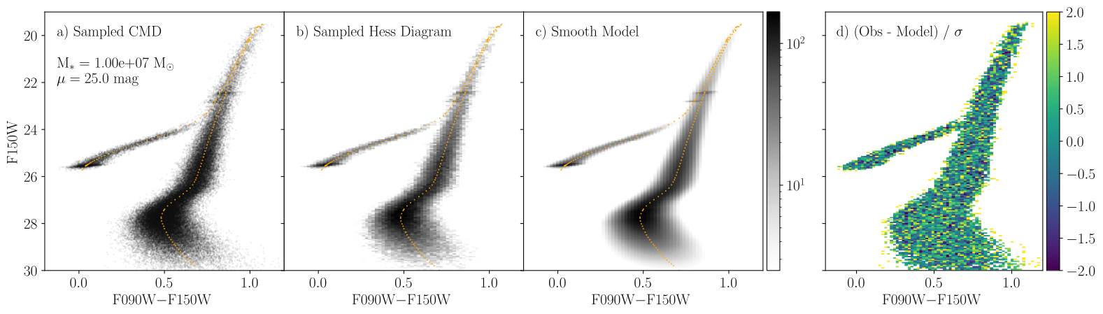
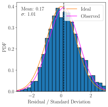
At left is a population of stars sampled from an SSP with the methods described in the section of the documentation on simulating CMDs. The points from the isochrone are colored orange. The next figure shows the binned Hess diagram derived from these data. The next figure shows our smooth Hess diagram template calculated for this SSP. The final figure at right shows the residual between the data and model in units of standard deviations. These are sometimes called Pearson residuals. Below we show the distribution of these residuals, which should be Gaussian with mean 0 and standard deviation 1 if the model were perfect. Note that, because all bins with 0 observed stars are excluded from the distribution and the observed Hess diagram contains Poisson error, the mean of our distribution will always be slightly higher than 0. We do, however, achieve a standard deviation of nearly 1, indicating that our model is robust. We show a Gaussian PDF with standard deviation 1 and mean equal to the observed mean of the residuals for comparison.
The method used to create these smooth Hess diagram templates is partial_cmd_smooth.
StarFormationHistories.partial_cmd_smooth — Function
result::StatsBase.Histogram =
    partial_cmd_smooth(m_ini::AbstractVector{<:Number},
                       mags::AbstractVector{<:AbstractVector{<:Number}},
                       mag_err_funcs,
                       y_index,
                       color_indices,
                       imf,
                       completeness_funcs=[one for i in mags],
                       bias_funcs=[zero for i in mags];
                       dmod::Number=0,
                       normalize_value::Number=1,
                       binary_model::AbstractBinaryModel=NoBinaries(),
                       mean_mass=mean(imf),
                       edges=nothing,
                       xlim=nothing,
                       ylim=nothing,
                       nbins=nothing,
                       xwidth=nothing,
                       ywidth=nothing)
Main function for generating template Hess diagrams from a simple stellar population of stars from an isochrone, including photometric error and completeness.
Arguments
m_ini::AbstractVector{<:Number}is a vector containing the initial stellar masses of the stars from the isochrone. The isochrone points must be in evolutionary order (e.g., in order of equivalent evolutionary points), as given by isochrone libraries; seeStarFormationHistories.ingest_isochrone.mags::AbstractVector{<:AbstractVector{<:Number}}is a vector of vectors. Each constituent vector with indexishould havelength(mags[i]) == length(m_ini), representing the magnitudes of the isochrone stars in each of the magnitudes considered. In most cases, mags should contain 2 (if y-axis mag is also involved in the x-axis color) or 3 vectors.mag_err_funcscomputes the 1σ photometric errors for the filters provided inmags. It is either aVectororTupleof callables (e.g., aFunction) with one callable per filter inmags, each taking a single apparent magnitude and returning aNumber, or a single joint callable as described in the "Joint Photometric Models" section below.y_indexgives a valid index (e.g., anIntorCartesianIndex) intomagsfor the filter you want to have on the y-axis of the Hess diagram. For example, if themagsargument contains the B and V band magnitudes asmags=[B, V]and you want V on the y-axis, you would sety_indexas2.color_indicesis a length-2 indexable object giving the indices intomagsthat are to be used to compute the x-axis color. For example, if themagsargument contains the B and V band magnitudes asmags=[B, V], and you want B-V to be the x-axis color, thencolor_indicesshould be[1,2]or(1,2)or similar.imfis a callable that takes an initial stellar mass as its sole argument and returns the (properly normalized) probability density of your initial mass function model. All the models from InitialMassFunctions.jl are valid forimf.completeness_funcsgives the completeness fractions as a function of apparent magnitude. It is either aVectororTupleof callables (e.g., aFunction) returning the single-filter completeness for the matching filter provided inmags, in which case the completeness of a star is the product of the single-filter completeness values in the filters used in the Hess diagram, or a single joint callable as described in the "Joint Photometric Models" section below.bias_funcsgives the expected photometric bias as a function of apparent magnitude. The photometric bias is defined as the difference between measured and intrinsic magnitude (i.e.,output - inputfor artificial star tests). It is either aVectororTupleof callables (e.g., aFunction) with one callable per filter inmags, or a single joint callable as described in the "Joint Photometric Models" section below.
Keyword Arguments
dmod::Number=0is the distance modulus in magnitudes to apply to the inputmags. Leave at0if you are providing apparent magnitudes inmags.normalize_value::Number=1is the total stellar mass of the population you wish to model.binary_model::AbstractBinaryModel=NoBinaries()is the model to use for including binary systems; seeStarFormationHistories.NoBinaries,StarFormationHistories.RandomBinaryPairs, andStarFormationHistories.BinaryMassRatio.mean_mass::Numberis the expectation value of the initial mass for a random star drawn from your providedimf. This will be computed for you if your providedimfis a valid continuous, univariateDistributions.Distributionobject.edgesis a tuple of ranges defining the left-side edges of the bins along the x-axis (edges[1]) and the y-axis (edges[2]). Example:(-1.0:0.1:1.5, 22:0.1:27.2). Ifedgesis provided, it overrides the following keyword arguments that offer other ways to specify the extent of the Hess diagram.xlimis a length-2 indexable object (e.g., aVectororTuple) giving the lower and upper bounds on the x-axis corresponding to the providedcolorsarray. Example:(-1.0, 1.5). This is only used ifedgesis not provided.ylimis asxlimbut for the y-axis corresponding to the providedmagsarray. Example(25.0, 20.0). This is only used ifedgesis not provided.nbins::NTuple{2, <:Integer}is a 2-tuple of integers providing the number of bins to use along the x- and y-axes. This is only used ifedgesis not provided.xwidthis the bin width along the x-axis for thecolorsarray. This is only used ifedgesandnbinsare not provided. Example:0.1.ywidthis asxwidthbut for the y-axis corresponding to the providedmagsarray. Example:0.1.
Returns
This method returns the Hess diagram as a StatsBase.Histogram; you should refer to the StatsBase documentation for more information. In short, if the output of this method is result, then the Hess diagram represented as a Matrix is available as result.weights (this is what you would want for fit_templates and similar functions) and the edges of the histogram are available as result.edges.
Joint Photometric Models
Per-filter models assume that the completeness, error, and bias in each filter depend only on the magnitude in that filter. This cannot represent, for example, a catalog cut requiring a minimum signal-to-noise ratio in every filter, which removes stars along a diagonal line in the Hess diagram. Each of mag_err_funcs, completeness_funcs, and bias_funcs may instead be a single joint callable that takes one apparent magnitude per filter in mags, in the same order as mags (e.g., f(mag_1, mag_2) for two filters). A joint completeness_funcs returns the probability that a star is detected and passes all selection criteria, and a joint mag_err_funcs or bias_funcs returns one value per filter (e.g., a Tuple or StaticArrays.SVector). Joint and per-filter models can be mixed; for example, a joint completeness model can be used with per-filter error and bias models. Photometric errors are still assumed to be uncorrelated between filters. See process_ASTs for measuring joint models from artificial star tests.
result::StatsBase.Histogram =
    partial_cmd_smooth(m_ini::AbstractVector{<:Number},
                       mags::AbstractVector{<:AbstractVector{<:AbstractVector{<:Number}}},
                       knots::AbstractVector{<:Number},
                       extinction::Distributions.ContinuousUnivariateDistribution,
                       mag_err_funcs, y_index, color_indices, imf,
                       completeness_funcs=[one for i in first(mags)],
                       bias_funcs=[zero for i in first(mags)];
                       max_shift::Real=0.5, kws...)
Method for a simple stellar population whose stars have a distribution of V-band extinctions extinction (differential extinction), for example a Distributions.Uniform for the model of MATCH [1] or the result of match_extinction. extinction is passed through prepare_extinction, so unbounded distributions are truncated and distributions with point masses are rejected.
mags[n] holds the isochrone magnitudes at extinction knots[n], in the same format as the mags argument of the method without extinction (one vector per filter, each with one entry per element of m_ini). The magnitudes are interpolated linearly in extinction between knots, so the knots should include every extinction at which the magnitudes are not linear, such as the extinction nodes of the bolometric correction grid (e.g., BolometricCorrections.Av_nodes), and must bracket the support of extinction. knots must be sorted.
Each isochrone point is deposited along its path through the Hess diagram as extinction increases, in sub-segments across which it moves by at most max_shift times the larger of its photometric error and the bin width. Each sub-segment is a Gaussian kernel whose covariance includes the spread of extinction across the sub-segment, with the photometric error, completeness, and bias evaluated at the mean extinction of the sub-segment. The template converges to the exact mixture of templates over extinction as max_shift decreases; the default of 0.5 is accurate enough for fits of $\sim 10^5$ stars. Other arguments and keyword arguments are as for the method without extinction, including binary models.
The user-provided functions returning magnitude errors (mag_err_funcs) and completeness values (completness_functions) given a star's intrinsic apparent magnitude are important for deriving good templates. These are typically derived from catalogs of artificial star tests. Some helper functions for constructing these are provided here.
Differential extinction
The stars of a population often have a range of extinctions rather than a single value, for example in star-forming regions of dusty galaxies. The method of partial_cmd_smooth that takes isochrone magnitudes at several extinctions (knots) and a distribution of V-band extinctions builds the template for such a population directly. Each isochrone point is moved along its reddening path through the Hess diagram in steps short enough that it moves by at most max_shift times the larger of its photometric error and the bin width, and each step is deposited as a Gaussian kernel broadened by the spread of extinction along it, with the photometric errors, completeness, and bias evaluated at the step's mean extinction. Magnitudes are interpolated linearly in extinction between knots, so the knots should include every extinction at which the magnitudes are not linear in extinction, such as the extinction nodes of the bolometric correction grid (BolometricCorrections.Av_nodes). For example, with an isochrone function iso(A) returning the initial masses and F475W and F814W magnitudes at extinction A,
using BolometricCorrections: Av_nodes
using Distributions: Uniform
extinction = Uniform(0.2, 1.2) # A_V uniformly distributed from 0.2 to 1.2 mag
knots = [0.2; filter(a -> 0.2 < a < 1.2, Av_nodes(bc_grid)); 1.2]
mags = [iso(a).mags for a in knots] # mags[n] = [F475W, F814W] at knots[n]
template = partial_cmd_smooth(iso(0.2).m_ini, mags, knots, extinction, mag_err_funcs, 2, (1, 2), imf,
                              completeness_funcs; dmod=dmod, edges=edges)
The model of differential extinction in MATCH [1], in which all stars have extinctions distributed uniformly between $A_V$ and $A_V + dA_V$ and young stars have an additional spread [3], is provided by match_extinction. ExponentialDiskExtinction generalizes it to stars and dust in exponential disks with different scale heights, e.g., young stars embedded in the dust layer or old stars in a thicker disk, most of which lie either in front of or behind a thin dust layer, and match_extinction can add the additional spread of young stars to it. Any other continuous distribution from Distributions.jl can also be used; prepare_extinction describes how unbounded distributions are truncated.
StarFormationHistories.match_extinction — Function
match_extinction(Av::Real, dAv::Real, dAvy::Real, logAge::Real; t1::Real=4e7, t2::Real=1e8)Returns the distribution of V-band extinctions for stars with logarithmic age logAge (log10(age [yr])) in the differential extinction model of MATCH [1]. Every star receives an extinction drawn uniformly from Av to Av + dAv, and stars younger than t2 years receive an independent additional extinction drawn uniformly from 0 to w(t) dAvy, where w(t) is 1 for ages below t1 and decreases linearly in age to 0 at t2 [3]. Returns a Distributions.Uniform when only one of the two terms is nonzero, and a UniformSum otherwise. Requires dAv + w(t) dAvy > 0.
match_extinction(base::Distributions.ContinuousUnivariateDistribution, dAvy::Real, logAge::Real;
                 t1::Real=4e7, t2::Real=1e8)
Adds the additional extinction of young stars, as above, to another distribution of extinctions base (e.g., an ExponentialDiskExtinction), returning base for stars older than t2 and a UniformConvolution otherwise.
julia> match_extinction(0.2, 0.6, 0.5, 9.0) == Uniform(0.2, 0.8) # older than t2; only dAv applies
true

julia> round.(extrema(match_extinction(0.2, 0.6, 0.5, 7.0)); digits=6) # younger than t1; both apply
(0.2, 1.3)StarFormationHistories.UniformSum — Type
UniformSum(a::Real, w1::Real, w2::Real)Distribution of X + Y for independent X ~ Uniform(a, a + w1) and Y ~ Uniform(0, w2), a trapezoid that rises from a over the smaller width, is flat, and falls to zero at a + w1 + w2 over the smaller width. This is the distribution of extinctions in the MATCH model of differential extinction for young stars; see match_extinction. Supports pdf, cdf, minimum, maximum, mean, var, and rand.
StarFormationHistories.ExponentialDiskExtinction — Type
ExponentialDiskExtinction(Av::Real, dAv::Real, s::Real; f_red::Real=1//2, σ::Real=0)Distribution of V-band extinctions for stars in a disk behind a foreground screen of extinction Av. The stars are embedded in a disk of dust with total extinction dAv. The stars and dust both have two-sided exponential vertical profiles, and the scale height of the stars is s times that of the dust. Each star has extinction Av + dAv U, where U is the fraction of the dust in front of it. The midplane of the dust is offset from that of the stars so that a fraction f_red of the stars lie behind it.
With s = 1 and f_red = 1/2 the stars and dust are perfectly mixed and the distribution is a uniform tophat between Av and Av + dAv, as in the model of MATCH [1]. For f_red = 1/2, U has density $[2 \, \text{min}(u, 1-u)]^{1/s - 1} / s$, which for s < 1 (stars embedded in the dust) peaks at u = 1/2 and for s > 1 diverges at u = 0 and u = 1, tending to equal point masses at both as s → ∞ (a thin dust layer).
With σ > 0, the total extinction of the dust varies across the face of the disk, as a log-normal distribution with median dAv and width σ in the natural logarithm, independent of the positions of the stars within the disk, as in the model of Dalcanton et al. [4]. The log-normal is truncated 3σ above its median, so the support is [Av, Av + dAv exp(3σ)], and pdf, cdf, quantile, and partial_mean are integrated numerically over it. In the limit of a thin dust layer, s → ∞, a fraction 1 - f_red of the stars has extinction Av and a fraction f_red has log-normally distributed extinction above it, as in that model. With the scale height ratios of young and old stars and their transition age, these are the parameters of the -diskav model of MATCH [5].
Supports pdf, cdf, quantile, minimum, maximum, mean, var, rand, and InitialMassFunctions.partial_mean.
julia> d = ExponentialDiskExtinction(0.2, 1.0, 3.0);

julia> extrema(d)
(0.2, 1.2)

julia> cdf(d, 0.7) # half of the stars lie in front of the dust midplane
0.5StarFormationHistories.UniformConvolution — Type
UniformConvolution(base::Distributions.ContinuousUnivariateDistribution, w::Real)Distribution of X + Y for independent X ~ base and Y ~ Uniform(0, w), e.g., the additional differential extinction of young stars in the model of MATCH [3] added to another distribution of extinctions; see match_extinction. base must be bounded. The density is at most 1 / w, so it is finite even where that of base is not. The cdf integrates the cdf of base, using InitialMassFunctions.partial_mean(base, x), which is integrated numerically unless base has a closed form, or directly for ExponentialDiskExtinction. Supports pdf, cdf, minimum, maximum, mean, var, and rand.
StarFormationHistories.prepare_extinction — Function
prepare_extinction(dist; nσ::Real=3)Checks that dist can be used as a distribution of V-band extinctions for partial_cmd_smooth and returns it, truncated if needed. dist must be a Distributions.ContinuousUnivariateDistribution; distributions with point masses (e.g., Distributions.Dirac) are not supported. A side of dist that is unbounded is truncated at the quantile that corresponds to nσ standard deviations of a normal distribution (a tail probability of about 0.00135 for nσ = 3), and the support is truncated at zero, as negative extinctions are unphysical. dist is returned unchanged if no truncation is needed.
julia> prepare_extinction(Uniform(0.2, 1.2)) == Uniform(0.2, 1.2)
true

julia> round.(extrema(prepare_extinction(Normal(0.7, 0.15))); digits=6)
(0.25, 1.15)We note that in many cases it can also be helpful to add in a foreground/background template that models contamination of the Hess diagram from stars not in your population of interest – this is often done using observations of parallel fields though there are several other possible methods.
Photometric catalogs can be processed into Hess diagrams meeting our formatting requirements with the method bin_cmd.
StarFormationHistories.bin_cmd — Function
result::StatsBase.Histogram =
   bin_cmd(colors::AbstractVector{<:Number},
           mags::AbstractVector{<:Number};
           weights::AbstractVector{<:Number} = ones(promote_type(eltype(colors),
                                                    eltype(mags)), size(colors)),
           edges  = nothing,
           xlim   = extrema(colors),
           ylim   = extrema(mags),
           nbins  = nothing,
           xwidth = nothing,
           ywidth = nothing)
Returns a StatsBase.Histogram type containing the Hess diagram from the provided x-axis photometric colors and y-axis photometric magnitudes mags. These must all be vectors equal in length. You can either specify the bin edges directly via the edges keyword (e.g., edges = (range(-0.5, 1.6, length=100), range(17.0, 26.0, length=100))), or you can set the x- and y-limits via xlim and ylim and the number of bins as nbins, or you can omit nbins and instead pass the bin width in the x and y directions, xwidth and ywidth. See below for more info on the keyword arguments. To plot this with PyPlot.jl you should do PyPlot.imshow(permutedims(result.weights), origin="lower", extent=(extrema(result.edges[1])..., extrema(result.edges[2]), kws...) where kws... are any other keyword arguments you wish to pass to PyPlot.imshow.
Keyword Arguments
weights::AbstractVector{<:Number}is a array of length equal tocolorsandmagsthat contains the probabilistic weights associated with each point. This is passed toStatsBase.fitasStatsBase.Weights(weights). The following keyword arguments are passed toStarFormationHistories.calculate_edgesto determine the bin edges of the histogram.edgesis a tuple of ranges defining the left-side edges of the bins along the x-axis (edges[1]) and the y-axis (edges[2]). Example:(-1.0:0.1:1.5, 22:0.1:27.2). Ifedgesis provided,weightsis the only other keyword that will be read;edgessupercedes the other construction methods.xlimis a length-2 indexable object (e.g., a vector or tuple) giving the lower and upper bounds on the x-axis corresponding to the providedcolorsarray. Example:[-1.0, 1.5]. This is only used ifedgesis not provided.ylimis likexlimbut for the y-axis corresponding to the providedmagsarray. Example[25.0, 20.0]. This is only used ifedgesis not provided.nbins::NTuple{2, <:Integer}is a 2-tuple of integers providing the number of bins to use along the x- and y-axes. This is only used ifedgesis not provided.xwidthis the bin width along the x-axis for thecolorsarray. This is only used ifedgesandnbinsare not provided. Example:0.1.ywidthis likexwidthbut for the y-axis corresponding to the providedmagsarray. Example:0.1.
Regions of the Hess diagram that are poorly modeled or contaminated (e.g., by foreground stars) can be excluded from a fit by removing their bins from both the observed Hess diagram and the templates. hess_mask returns the bins inside a set of polygons for this purpose.
StarFormationHistories.hess_mask — Function
hess_mask(edges, gates)::BitMatrixReturns a mask for a Hess diagram with bin edges edges (e.g., (xedges, yedges) as used by bin_cmd) that is true for bins whose centers lie inside any of the polygons in gates. Each polygon is a vector of (x, y) vertices in the coordinates of the Hess diagram (e.g., color and magnitude). Polygons are closed automatically, so the last vertex need not repeat the first, and may be concave.
Removing the masked bins from both the observed Hess diagram and the templates excludes these regions from a fit, as they then contribute nothing to the likelihood. This is equivalent to the "gates" of the MATCH software. With the flattened layout from stack_models, this can be done for any of the fitting methods as
keep = .!vec(hess_mask(edges, gates))
fit_templates(stack_models(models)[keep, :], vec(data)[keep])A Note on Array Formatting
It is expected that the user will typically have model templates stored as two-dimensional matrices as these are the obvious choice for representing a binned two-dimensional histogram. We fully support supplying the list of model templates as a list of matrices (e.g., a Vector{Matrix{<:Number}}) to the fitting functions discussed below. The important computational kernels composite! and ∇loglikelihood! have custom loops for these input types.
However, additional optimizations are possible by flattening the data. By flattening each matrix in the list of model templates into a column vector and concatenating them such that the list of model templates becomes a single matrix, we can compute the complex model Hess diagram as a single matrix-vector product rather than using a custom loop. The same optimization can be made when computing the gradient of the loglikelihood (discussed more below). The majority of all computation for the fitting methods below is spent in these two functions, so optimizing their performance translates directly to improved fitting runtimes. With this flattened memory arrangement we can use the highly optimized LinearAlgbera.mul! method to do the in-place matrix-vector product. This will typically be translated into a call to a BLAS function like gemv!. As such, we can benefit from Julia's ability to switch BLAS implementations at runtime to use Intel's Math Kernel Library, Apple's Accelerate, and others.
Most of the fitting methods below support both the natural and flattened data layouts. We provide the stack_models method to produce the optimized layout for the list of model templates.
StarFormationHistories.stack_models — Function
stack_models(models::AbstractVector{<:AbstractMatrix{<:Number}})Transforms a vector of matrices into a single matrix, with each matrix from models being transcribed into a single column in the output matrix. This data layout enables more efficient calculations in some of our internal functions like composite! and ∇loglikelihood!. This function is just reduce(hcat, map(vec, models)).
Examples
julia> stack_models([rand(5,5) for i in 1:10])
25×10 Matrix{Float64}:
...A Note on Threading
While generally the methods using BLAS routines offer significant performance improvements, there is a caveat when multithreading from within Julia. By default Julia will allow BLAS to use multiple threads even if Julia itself is started with a single thread (i.e., by running julia -t 1). BLAS threads do not compose with Julia threads. That is, if you start Julia with N>1 threads (julia -t N) and write a threaded workload where each Julia thread is doing BLAS operations concurrently, you can easily oversubscribe the CPU. Specific recommendations vary depending on BLAS vendor (see this page and the linked discourse threads), but generally this package is in the regime of doing many small calculations that do not individually benefit much from BLAS threading (e.g., performance for OpenBLAS with 8 threads is only ~2x the 1 thread performance). As such it is often sufficient to set BLAS to use a single thread (via LinearAlgbera.BLAS.set_num_threads(1) or environment variables; see above link).
References
- [1]
- A. Dolphin. Numerical methods of star formation history measurement and applications to seven dwarf spheroidals. MNRAS 332, 91–108 (2002), arXiv:astro-ph/0112331 [astro-ph].
- [2]
- D. R. Weisz, A. E. Dolphin, A. Savino, K. B. McQuinn, M. J. Newman, B. F. Williams, N. Kallivayalil, J. Anderson, M. L. Boyer, M. Correnti, M. C. Geha, K. M. Sandstrom, A. A. Cole, J. T. Warfield, E. D. Skillman, R. E. Cohen, R. Beaton, A. Bressan, A. Bolatto, M. Boylan-Kolchin, A. M. Brooks, J. S. Bullock, C. Conroy, M. C. Cooper, J. J. Dalcanton, A. L. Dotter, T. K. Fritz, C. T. Garling, M. Gennaro, K. M. Gilbert, L. Girardi, B. D. Johnson, L. C. Johnson, J. Kalirai, E. N. Kirby, D. Lang, P. Marigo, H. Richstein, E. F. Schlafly, E. J. Tollerud and A. Wetzel. The JWST Resolved Stellar Populations Early Release Science Program. V. DOLPHOT Stellar Photometry for NIRCam and NIRISS. ApJS 271, 47 (2024), arXiv:2402.03504 [astro-ph.GA].
- [3]
- A. E. Dolphin, A. Saha, E. D. Skillman, R. Dohm-Palmer, E. Tolstoy, A. Cole, J. Gallagher, J. Hoessel and M. Mateo. Deep Hubble Space Telescope Imaging of Sextans A. III. The Star Formation History. AJ 126, 187–196 (2003), arXiv:astro-ph/0304098.
- [4]
- J. J. Dalcanton, M. Fouesneau, D. W. Hogg, D. Lang, A. K. Leroy, K. D. Gordon, K. Sandstrom, D. R. Weisz, B. F. Williams, E. F. Bell, H. Dong, K. M. Gilbert, D. A. Gouliermis, P. Guhathakurta, T. R. Lauer, A. Schruba, A. C. Seth and E. D. Skillman. The Panchromatic Hubble Andromeda Treasury. VIII. A Wide-area, High-resolution Map of Dust Extinction in M31. ApJ 814, 3 (2015), arXiv:1509.06988 [astro-ph.GA].
- [5]
- B. F. Williams, A. E. Dolphin, J. J. Dalcanton, D. R. Weisz, E. F. Bell, A. R. Lewis, P. Rosenfield, Y. Choi, E. Skillman and A. Monachesi. PHAT. XIX. The Ancient Star Formation History of the M31 Disk. ApJ 846, 145 (2017).