BaSTIv2

Here we describe the interface we provide to the updated BaSTI stellar models presented in [21, 24–26]. BaSTIv2 specific code is housed in the BaSTIv2 submodule, which can be accessed as

using StellarTracks.BaSTIv2 # load all exported methods
using StellarTracks.BaSTIv2: BaSTIv2Library, X, Y, Z # load specific methods

Data Acquisition

The tracks are distributed as a lazy Julia artifact that is downloaded automatically the first time you try to access them. The main access point we provide is BaSTIv2Library, which will load and make available a set of stellar models corresponding to a specific chemical mixture and set of input physics. The total data volume is ~150 MB. The data are tied to the installed version of StellarTracks.jl and are removed by Julia's package garbage collector (using Pkg; Pkg.gc(), which also runs automatically during package updates) once no installed version of StellarTracks.jl uses them. Versions of StellarTracks.jl before v1.2 downloaded these tracks with DataDeps.jl. That copy is no longer used; if it was saved in the default DataDeps location, it can be removed with

rm(joinpath(DEPOT_PATH[1], "scratchspaces", "124859b0-ceae-595e-8997-d05f6a7a8dfe", "datadeps", "BaSTIv2"); recursive=true, force=true)

With all the tracks available, we are able to perform operations like interpolating isochrones at any age and metallicity within the BaSTIv2 parameter space.

Grid Properties

The BaSTIv2 model grid contains models for the following iron abundances:

println(BaSTIv2.feh_grid)

[-3.2, -2.5, -2.2, -1.9, -1.7, -1.55, -1.4, -1.3, -1.2, -1.05, -0.9, -0.7, -0.6, -0.4, -0.3, -0.2, -0.1, 0.06, 0.15, 0.3, 0.45]

This is a superset of all available iron abundances; not all combinations of physics and chemistry will have all these iron abundances available. In particular, the α-enhanced models with [α/Fe]=0.4 presently have a limited number of iron abundances available.

The BaSTIv2 grid includes models with scaled-solar abundance patterns, α-enhanced models with an average [α/Fe]=0.4 (presented in Pietrinferni et al. [24]), and α-depleted models with [α/Fe]=-0.2 (presented in Pietrinferni et al. [26]. For these models, the abundances of the α elements O, Ne, Mg, Si, S, Ar, Ca, and Ti have been changed relative to Fe. These α-enhanced models are useful for modeling low-metallicity stars that formed prior to significant iron enrichment from type Ia supernovae. These stars are most common in the Galactic halo and low-mass dwarf galaxies. Note that the conversion between metal mass fraction $Z$ and logarithmic metal abundance [M/H] is the same for the scaled-solar models as for the α-enhanced models, however the iron abundance [Fe/H] is not the same as [M/H] – see Table 1 of Pietrinferni et al. [24] and Pietrinferni et al. [26] for the full elemental abundance tables.

For scaled-solar abundance patterns, models are available with different physics models varying convective overshooting during central H-burning and atomic diffusion. So-called "canonical" models do not including overshooting, while "non-canonical" models do include a convective overshooting treatment (see section 3 of Pietrinferni et al. [18]). Inclusion of convective overshooting during central H-burning mainly changes the main sequence turn-off morphology and generally results in better fits to simple stellar populations like globular clusters. For methods in this module that take a canonical::Bool argument, a value of canonical=true indicates you want to use the "canonical" stellar models, while a value of canonical=false means you want to use the "non-canonical" models that include convective core overshooting. Similarly, setting an argument diffusion::Bool=true indicates you wish to use the models with atomic diffusion. For scaled-solar abundance patterns, models with different Reimers mass loss parameters η are also available.

The α-depleted [26] and α-enhanced [24] models are only available with overshooting and diffusion (canonical=false, diffusion=true, with η=0.3). Additional α-enhanced models with enhanced primordial helium abundances are also available (yp = 0.247 (fiducial), 0.275, 0.3, 0.32).

Not all combinations of canonical, diffusion, α-element abundance, primordial helium abundance yp, and Reimers mass loss parameter η are valid. The table below summarizes the available combinations of parameters.

[α/Fe]	canonical	diffusion	yp	η
-0.2	false	true	0.247	0.3
0.0	false	true	0.247	0.3
0.0	false	false	0.247	0.0
0.0	false	false	0.247	0.3
0.0	true	false	0.247	0.0
0.4	false	true	0.247	0.3
0.4	false	true	0.275	0.3
0.4	false	true	0.300	0.3
0.4	false	true	0.320	0.3

As setting up these arguments can be arduous, we have attempted to provide useful error messages when an invalid combination of arguments is requested.

Examples

First we load the scaled-solar models ([α/Fe] = 0.0) with convective core overshooting (canonical = false), diffusion (diffusion = true), primordial helium abundance yp = 0.247, and Reimers mass loss parameter η = 0.3. These models will be downloaded if not already available.

using StellarTracks.BaSTIv2
p = BaSTIv2Library(0.0, false, true, 0.247, 0.3)

Structure of interpolants for the updated BaSTI library of non-canonical stellar tracks with diffusion, [α/Fe]=0.0, Y_p=0.247, η=0.3. Valid range of metallicities is [Fe/H] = (-3.2, 0.3), [M/H] = (-3.2, 0.3).

Now we use the BaSTIv2Library to interpolate an isochrone at log10(age [yr]) = 10.05 and logarithmic metallicity [M/H] = -1.234. The isochrone is returned as a NamedTuple.

iso = isochrone(p, 10.05, -1.234)

(eep = [62, 63, 64, 65, 66, 67, 68, 69, 70, 71  …  2091, 2092, 2093, 2094, 2095, 2096, 2097, 2098, 2099, 2100], m_ini = [0.10207219574497858, 0.10509923836482174, 0.10729312254052467, 0.10902387204273777, 0.11045782669185918, 0.11168459742613916, 0.11275817642484944, 0.1137136909790877, 0.1145753157558331, 0.11536041884270352  …  0.8388585192444433, 0.8388598694011791, 0.8388612195654495, 0.8388625697413018, 0.8388639199206402, 0.8388652701096649, 0.8388666203052642, 0.8388679705116127, 0.8388693207222799, 0.838870670941439], logTe = [3.501151394410137, 3.5084220173539626, 3.5135025247990583, 3.517339390785174, 3.520382719473182, 3.522878668831519, 3.5249754335225343, 3.5267669807789894, 3.5283182739435928, 3.52967607382725  …  3.64812965327389, 3.6470421224526874, 3.6458552601766137, 3.6444952088811635, 3.643112335510638, 3.6416191816936045, 3.63997841945088, 3.6381954749042404, 3.6366110488701087, 3.6349265163479587], Mbol = [12.06185831350745, 11.928103838774703, 11.833199580856014, 11.761079037873326, 11.703387487179667, 11.655526658597811, 11.614776135807524, 11.579439207708369, 11.548367886107851, 11.520727546729997  …  -2.217006441615966, -2.2529417565506833, -2.290586700649727, -2.331715131131252, -2.3749483406998397, -2.4191553496868616, -2.465828223345076, -2.515602322790107, -2.564780245080494, -2.6151773903828213], logg = [5.334779151930746, 5.322779402530015, 5.313970386748252, 5.307329063280509, 5.30205044519346, 5.297668133148366, 5.29391546525461, 5.2906366848265, 5.2877315298796965, 5.28512514954891  …  1.0542998488010982, 1.0358558541546727, 1.0164553856685747, 0.9951121112957264, 0.972901379578166, 0.9499641176067602, 0.9254987791023871, 0.899264808604314, 0.873520759331746, 0.8468504736499495], logL = [-2.9287433254029795, -2.8752415355098813, -2.8372798323424058, -2.8084316151493303, -2.7853549948718674, -2.766210663439124, -2.749910454323009, -2.7357756830833484, -2.723347154443141, -2.712291018691999  …  2.782802576646387, 2.797176702620273, 2.8122346802598903, 2.8286860524525013, 2.845979336279936, 2.863662139874745, 2.88233128933803, 2.902240929116043, 2.9219120980321973, 2.9420709561531284])

The NamedTuple returned by isochrone can be converted to table types, like TypedTables.Table to simplify further use.

using TypedTables: Table
Table(iso)

Table with 6 columns and 2039 rows:
      eep  m_ini     logTe    Mbol     logg     logL
    ┌───────────────────────────────────────────────────
 1  │ 62   0.102072  3.50115  12.0619  5.33478  -2.92874
 2  │ 63   0.105099  3.50842  11.9281  5.32278  -2.87524
 3  │ 64   0.107293  3.5135   11.8332  5.31397  -2.83728
 4  │ 65   0.109024  3.51734  11.7611  5.30733  -2.80843
 5  │ 66   0.110458  3.52038  11.7034  5.30205  -2.78535
 6  │ 67   0.111685  3.52288  11.6555  5.29767  -2.76621
 7  │ 68   0.112758  3.52498  11.6148  5.29392  -2.74991
 8  │ 69   0.113714  3.52677  11.5794  5.29064  -2.73578
 9  │ 70   0.114575  3.52832  11.5484  5.28773  -2.72335
 10 │ 71   0.11536   3.52968  11.5207  5.28513  -2.71229
 11 │ 72   0.116082  3.53087  11.4959  5.28277  -2.70237
 12 │ 73   0.11675   3.53194  11.4735  5.28062  -2.6934
 13 │ 74   0.117371  3.53289  11.4531  5.27865  -2.68524
 14 │ 75   0.117953  3.53374  11.4344  5.27683  -2.67778
 15 │ 76   0.1185    3.53451  11.4173  5.27515  -2.67092
 16 │ 77   0.119016  3.53521  11.4015  5.2736   -2.6646
 17 │ 78   0.119505  3.53584  11.3869  5.27214  -2.65875
 ⋮  │  ⋮      ⋮         ⋮        ⋮        ⋮        ⋮

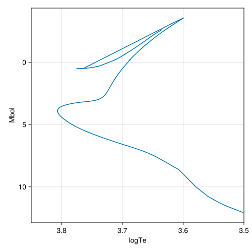
The theoretical isochrone is plotted below.

We can load a grid of bolometric corrections from BolometricCorrections.jl to add observational magnitudes to the theoretical isochrone. In this example, we use the MIST bolometric correction grid, which offers bolometric corrections for varying metallicities ([M/H]) and reddening values ($A_V$).

Because the solar metallicity calibrations of BaSTIv2 and MIST are not exactly the same, the protostellar metal mass fraction $Z$ that corresponds to a given [M/H] is not the same between the two libraries. The isochrone interface will convert the given [M/H], which is assumed to be the desired metallicity in the stellar track library, to its corresponding metal mass fraction, and then convert from the metal mass fraction to the correct [M/H] for the assumed chemical model of the bolometric correction grid. This Z-matched approach is appropriate because isochrones computed at equal total metallicity (equal Z) appear very similar across different α-enhancement levels, while isochrones at equal [Fe/H] can differ substantially when [α/Fe] varies (see, e.g., [17]).

This method returns a TypedTables.Table that contains the information from both sources. Here we evaluate an isochrone with log10(age [yr]) = 10.05, [M/H] = -1.234, and $A_v = 0.02$ mag.

using BolometricCorrections.MIST: MISTv1BCGrid
m = MISTv1BCGrid("JWST")
iso = isochrone(p, m, 10.05, -1.234, 0.02)

Table with 35 columns and 2039 rows:
      eep  m_ini     logTe    Mbol     logg     logL      F070W    F090W    ⋯
    ┌────────────────────────────────────────────────────────────────────────
 1  │ 62   0.102072  3.50115  12.0619  5.33478  -2.92874  12.3678  11.1373  ⋯
 2  │ 63   0.105099  3.50842  11.9281  5.32278  -2.87524  12.19    11.017   ⋯
 3  │ 64   0.107293  3.5135   11.8332  5.31397  -2.83728  12.0636  10.9256  ⋯
 4  │ 65   0.109024  3.51734  11.7611  5.30733  -2.80843  11.9674  10.8561  ⋯
 5  │ 66   0.110458  3.52038  11.7034  5.30205  -2.78535  11.8905  10.8006  ⋯
 6  │ 67   0.111685  3.52288  11.6555  5.29767  -2.76621  11.8268  10.7544  ⋯
 7  │ 68   0.112758  3.52498  11.6148  5.29392  -2.74991  11.7726  10.7152  ⋯
 8  │ 69   0.113714  3.52677  11.5794  5.29064  -2.73578  11.7257  10.6811  ⋯
 9  │ 70   0.114575  3.52832  11.5484  5.28773  -2.72335  11.6846  10.6511  ⋯
 10 │ 71   0.11536   3.52968  11.5207  5.28513  -2.71229  11.6482  10.6245  ⋯
 11 │ 72   0.116082  3.53087  11.4959  5.28277  -2.70237  11.6156  10.6005  ⋯
 12 │ 73   0.11675   3.53194  11.4735  5.28062  -2.6934   11.5862  10.5789  ⋯
 13 │ 74   0.117371  3.53289  11.4531  5.27865  -2.68524  11.5596  10.5592  ⋯
 14 │ 75   0.117953  3.53374  11.4344  5.27683  -2.67778  11.5353  10.5411  ⋯
 15 │ 76   0.1185    3.53451  11.4173  5.27515  -2.67092  11.5131  10.5245  ⋯
 16 │ 77   0.119016  3.53521  11.4015  5.2736   -2.6646   11.4927  10.5093  ⋯
 17 │ 78   0.119505  3.53584  11.3869  5.27214  -2.65875  11.4739  10.4951  ⋯
 ⋮  │  ⋮      ⋮         ⋮        ⋮        ⋮        ⋮         ⋮        ⋮     ⋱

All available columns in the isochrone can be obtained with TypedTables.columnnames.

using TypedTables: columnnames
columnnames(iso)

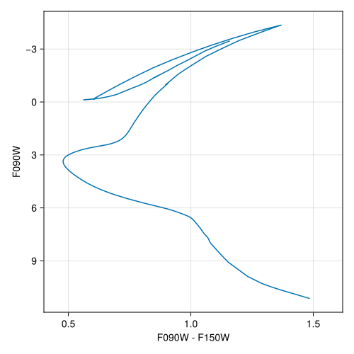
(:eep, :m_ini, :logTe, :Mbol, :logg, :logL, :F070W, :F090W, :F115W, :F140M, :F150W2, :F150W, :F162M, :F164N, :F182M, :F187N, :F200W, :F210M, :F212N, :F250M, :F277W, :F300M, :F322W2, :F323N, :F335M, :F356W, :F360M, :F405N, :F410M, :F430M, :F444W, :F460M, :F466N, :F470N, :F480M)

A color-magnitude diagram constructed from the isochrone is plotted below.

Chemistry API

We provide the StellarTracks.BaSTIv2.BaSTIv2Chemistry type that follows the chemistry API defined in BolometricCorrections.jl to access information on the chemical mixture assumed for the BaSTIv2 models.

StellarTracks.BaSTIv2.BaSTIv2Chemistry — Type

BaSTIv2Chemistry(α_fe::Number, yp::Number)

Returns a struct representing the BaSTIv2 chemical mixture model with [α/Fe] = α_fe and primordial helium abundance yp. These BaSTI models, presented in Hidalgo et al. [21], Pietrinferni et al. [24], Salaris et al. [25] and Pietrinferni et al. [26], include solar-scaled chemical compositions, α-enhanced compositions with [α/Fe] ≈ 0.4, and α-depleted compositions with [α/Fe] ≈ -0.2.

The solar protostellar chemical mixture for these models was calibrated to reproduce solar photospheric observations via a forward modeling approach (see section 3 of Hidalgo et al. [21]). Most solar photospheric abundances are taken from Caffau et al. [27].

As the BaSTIv2 grid was run with uniform [Fe/H] values but differing [α/Fe], the metal mass fraction $Z$ and the logarithmic metal abundance [M/H] are not uniform for every [α/Fe] in the grid. We therefore need to know [α/Fe] so that we can convert the [Fe/H] values to [M/H] and $Z$. The α-enhanced library also includes models with enhanced primordial helium abundance (yp here), so we require that information as well.

For the [α/Fe] = 0.4 models presented in Pietrinferni et al. [24] and the [α/Fe] = -0.2 models presented in Pietrinferni et al. [26], the α elements O, Ne, Mg, Si, S, Ca, and Ti have all been uniformly modified with respect to the Fe abundance relative to the Caffau et al. [27] heavy element distribution. As C and N are not changed, [M/H] = [Fe/H] + 0.75 * [α/Fe]; see, e.g., Equation 4 of Vazdekis et al. [22].

julia> using StellarTracks.BaSTIv2: BaSTIv2Chemistry, X, Y, Z, X_phot, Y_phot, Z_phot, MH;

julia> chem = BaSTIv2Chemistry(0.0, 0.247);

julia> X(chem) + Y(chem) + Z(chem) ≈ 1 # solar protostellar values
true

julia> X_phot(chem) + Y_phot(chem) + Z_phot(chem) ≈ 1 # solar photospheric values
true

julia> isapprox(MH(chem, Z_phot(chem) * 0.1), -1; atol=0.01)
true

julia> isapprox(Z(chem, -1), Z_phot(chem) * 0.1; rtol=0.02)
true

source

Note that in our conversions between $Z$ and [M/H], remembering that MH = log10(Z/X) - log10(Z⊙/X⊙), we use the photospheric solar values for Z⊙ and X⊙ (these are defined in section 3 of Hidalgo et al. [21]). This reproduces the relation between Z and [M/H] defined in Table 2 of Hidalgo et al. [21].

Library API

StellarTracks.BaSTIv2.BaSTIv2Library — Type

BaSTIv2Library(α_fe::Number=0, canonical::Bool=false, diffusion::Bool=true,
               yp::Number=0.247, η::Number=0.3)

BaSTIv2Library implements the AbstractTrackLibrary interface for the updated BaSTI stellar evolution models presented in [21, 24–26].

Optional Arguments

α_fe::Number = 0: [α/Fe] of stellar model.
canonical::Bool = false: Whether to use models with convective overshooting (false) or without (true).
diffusion::Bool = true: Whether to use models with atomic diffusion (true) or without (false).
yp::Number = 0.247: Primordial helium abundance assumed for stellar model.
η::Number = 0.3: Reimers mass loss parameter used to calculate the stellar model.

If you construct an instance as p = BaSTIv2Library(0.0, false), it is callable as p(mh::Number, M::Number) which returns an InterpolatedTrack that interpolates between tracks to a specific metallicity ([M/H]) and initial stellar mass (M).

This type also supports isochrone construction (see isochrone).

julia> p = BaSTIv2Library(0.0, false, true, 0.247, 0.3)
Structure of interpolants for the updated BaSTI library of non-canonical stellar tracks with diffusion, [α/Fe]=0.0, Y_p=0.247, η=0.3. Valid range of metallicities is [Fe/H] = (-3.2, 0.3), [M/H] = (-3.2, 0.3).

julia> isochrone(p, 10.05, -2.01) isa NamedTuple
true

julia> p(-2.05, 1.05)
InterpolatedTrack with M_ini=1.05, MH=-2.05, Z=0.000139413, Y=0.247183, X=0.752678.

source

StellarTracks.isochrone — Method

isochrone(p::BaSTIv2Library, logAge::Number, mh::Number)

Interpolates properties of the stellar tracks in the library at the requested logarithmic age (logAge = log10(age [yr])) and logarithmic metallicity [M/H] = mh. Returns a NamedTuple containing the properties listed below:

eep: Equivalent evolutionary points.
m_ini: Initial stellar masses, in units of solar masses.
logTe: Base-10 logarithm of the effective temperature [K] of the stellar model.
Mbol: Bolometric luminosity of the stellar model.
logg: Surface gravity of the stellar model.

source

The full library is principally a set of BaSTIv2TrackSets, with one track set per unique chemical composition. We do not presently offer interpolation as a function of [α/Fe] or between the canonical and non-canonical models, or between the models with and without diffusion, so the individual track sets in the library vary only in total metallicity (i.e., $Z$).

Track Set API

StellarTracks.BaSTIv2.BaSTIv2TrackSet — Type

BaSTIv2TrackSet(feh::Number, α_fe::Number=0, canonical::Bool=false,
                diffusion::Bool=true, yp::Number=0.247, η::Number=0.3)

BaSTIv2TrackSet implements the AbstractTrackSet interface for the updated BaSTI stellar evolution library [21, 24–26].

Arguments

feh::Number: [Fe/H] of stellar model

Optional Arguments

α_fe::Number = 0: [α/Fe] of stellar model.
canonical::Bool = false: Whether to use models with convective overshooting (false) or without (true).
diffusion::Bool = true: Whether to use models with atomic diffusion (true) or without (false).
yp::Number = 0.247: Primordial helium abundance assumed for stellar model.
η::Number = 0.3: Reimers mass loss parameter used to calculate the stellar model.

julia> ts = StellarTracks.BaSTIv2.BaSTIv2TrackSet(-2.2, 0.0, false, true, 0.247, 0.3)
Non-canonical BaSTIv2TrackSet with diffusion, [M/H]=-2.2, [Fe/H]=-2.2, [α/Fe]=0.0, Z=9.87095e-5, Y=0.247129, Y_p=0.247, η=0.3, 2099 EEPs and 56 initial stellar mass points.

julia> ts(1.01) # Interpolate track at new initial mass
Non-canonical BaSTIv2Track with diffusion, M_ini=1.01, [M/H]=-2.2, [Fe/H]=-2.2, [α/Fe]=0.0, Z=9.87095e-5, Y=0.247129, X=0.752772, Y_p=0.247, η=0.3.

julia> isochrone(ts, 10.0) isa NamedTuple # Interpolate isochrone at `log10(age [yr]) = 10`
true

source

Individual Tracks API

StellarTracks.BaSTIv2.BaSTIv2Track — Type

BaSTIv2Track(feh::Number, mass::Number, α_fe::Number, canonical::Bool, diffusion::Bool, yp::Number, η::Number)

BaSTIv2Track implements the AbstractTrack interface for the updated BaSTI stellar evolution library [21, 24–26].

Note that due to the organization of the BaSTIv2 data files, this method requires constructing a BaSTIv2TrackSet and is therefore not efficient if your aim is to construct multiple tracks with the same properties but different masses. In this case, you should construct a BaSTIv2TrackSet and call it with the masses you want, e.g., ts = BaSTIv2TrackSet(-2.2, 0.0, false, true, 0.247, 0.3); ts.([0.61, 0.82]).

Arguments

feh::Number: [Fe/H] of stellar model.
mass::Number: Initial stellar mass of stellar model in solar masses.
α_fe::Number: [α/Fe] of stellar model.
canonical::Bool: Whether to use models with convective overshooting (false) or without (true).
diffusion::Bool: Whether to use models with atomic diffusion (true) or without (false).
yp::Number: Primordial helium abundance assumed for stellar model.
η::Number: Reimers mass loss parameter used to calculate the stellar model.

Note that this function takes the input metallicity as [Fe/H], which is not equal to [M/H] when considering models with [α/Fe] != 0 α_fe != 0.

julia> track = StellarTracks.BaSTIv2.BaSTIv2Track(-2.2, 0.81, 0.0, false, true, 0.247, 0.3)
Non-canonical BaSTIv2Track with diffusion, M_ini=0.81, [M/H]=-2.2, [Fe/H]=-2.2, [α/Fe]=0.0, Z=9.87095e-5, Y=0.247129, X=0.752772, Y_p=0.247, η=0.3.

julia> track(9.0) # interpolate track at log10(age [yr]) = 9
(log_L = -0.13623875349579812, log_Teff = 3.801177574986798, log_g = 4.642108911103173)

source

Acknowledgements

We would like to thank Alessandro Savino for his assistance acquiring and working with the updated BaSTI tracks.

BaSTIv2 References

This page cites the following references:

[17]: M. Salaris, A. Chieffi and O. Straniero. The alpha-enhanced Isochrones and Their Impact on the FITS to the Galactic Globular Cluster System. ApJ 414, 580 (1993).
[18]: A. Pietrinferni, S. Cassisi, M. Salaris and F. Castelli. A Large Stellar Evolution Database for Population Synthesis Studies. I. Scaled Solar Models and Isochrones. ApJ 612, 168–190 (2004).
[21]: S. L. Hidalgo, A. Pietrinferni, S. Cassisi, M. Salaris, A. Mucciarelli, A. Savino, A. Aparicio, V. S. Aguirre and K. Verma. The Updated BaSTI Stellar Evolution Models and Isochrones. I. Solar-scaled Calculations. ApJ 856, 125 (2018).
[22]: A. Vazdekis, P. Coelho, S. Cassisi, E. Ricciardelli, J. Falcón-Barroso, P. Sánchez-Blázquez, F. La Barbera, M. Beasley and A. Pietrinferni. Evolutionary stellar population synthesis with MILES - II. Scaled-solar and α-enhanced models. MNRAS 449, 1177–1214 (2015), arXiv:1504.08032 [astro-ph.GA].
[24]: A. Pietrinferni, S. Hidalgo, S. Cassisi, M. Salaris, A. Savino, A. Mucciarelli, K. Verma, V. Silva Aguirre, A. Aparicio and J. W. Ferguson. Updated BaSTI Stellar Evolution Models and Isochrones. II. α-enhanced Calculations. ApJ 908, 102 (2021). Accessed on Apr 28, 2024. ADS Bibcode: 2021ApJ...908..102P.
[25]: M. Salaris, S. Cassisi, A. Pietrinferni and S. Hidalgo. The updated BASTI stellar evolution models and isochrones - III. White dwarfs. MNRAS 509, 5197–5208 (2022). Accessed on Apr 28, 2024. ADS Bibcode: 2022MNRAS.509.5197S.
[26]: A. Pietrinferni, M. Salaris, S. Cassisi, A. Savino, A. Mucciarelli, D. Hyder and S. Hidalgo. The updated BaSTI stellar evolution models and isochrones - IV. α-Depleted calculations. MNRAS 527, 2065–2070 (2024). Accessed on Apr 28, 2024. ADS Bibcode: 2024MNRAS.527.2065P.
[27]: E. Caffau, H.-G. Ludwig, M. Steffen, B. Freytag and P. Bonifacio. Solar Chemical Abundances Determined with a CO5BOLD 3D Model Atmosphere. Solar Physics 268, 255–269 (2011).